Implementing Belcour's Thin-Film BRDF

For this final project, I’ve implemented Belcour and Pascal’s thin-film BRDF in the La Jolla renderer. This write-up serves as a compilation of everything I learned while understanding and implementing the thin-film BRDF model. I began by studying the physical models governing the reflection and refraction of waves, then Belcour and Pascal’s specific approach, and finally rendered images demonstrating results similar to the real-life effect seen in differentially tempered steel.

Motivation

In the lecture where we discussed the Disney BSDFs, I encountered the concept of the complex index of refraction for the first time. Although we only used Schlick’s approximation in the Disney BSDF, it made me curious about what exactly a complex index of refraction signifies and how it arises physically.

Around the middle of the quarter, I became very interested in exploring visual phenomena arising from the wave nature of light. During this period, I briefly reviewed Belcour’s thin-film BRDF paper but didn’t delve deeply into its details. However, when choosing among the final project options, I decided to revisit and thoroughly study this topic.

Since rendering is relatively new to me, I had to rely on numerous references, videos, blogs, and lecture notes to understand the paper fully. Unfortunately, I did not consistently keep track of all these sources. Nevertheless, some key resources that I frequently returned to were the original paper A Practical Extension to Microfacet Theory for the Modeling of Varying Iridescence, lecture notes on WAVES by Prof. Matthew D. Schwartz, and a few of Bob Eagle’s lectures on Electricity and Magnetism on YouTube.

I’ve structured this report in the sequence I personally would have preferred when first learning these concepts. The high-level structure begins with discussing the underlying physics, followed by rendering theory, and concluding with implementation details.

Physical Model for Thin-Film Interference

This was definitely the most interesting part—though it also turned into quite the rabbit hole! Still, it was incredibly satisfying to see how closely the rendered effects matched the real-life reference from Wikipedia, especially after implementing these dense and convoluted equations.

Light as a Wave

For most rendering and ray tracing, we rely on geometric optics, which models light as a ray traveling in a straight line. But this is only an approximation of light’s wave nature, valid when any obstacles are much larger than the wavelength of light. Because of this approximation, it doesn’t capture phenomena like interference—which is the main reason behind the colorful patterns produced by thin films.

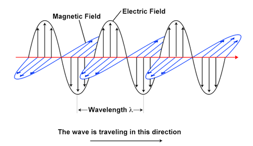
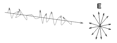
Even though the magnetic field is perpendicular to the electric field, the electric field can oscillate in any direction; when that direction varies randomly, the light is called unpolarized:

When we talk about light getting reflected and refracted, it’s just a light wave changing medium. At the boundary of these media we see the interesting changes in the wave properties which we classify as reflection and refraction. The equations which define it are called Fresnel equations, which are also the core part of the Cook–Torrance BRDF.

As light is an electromagnetic wave, there are four differential equations—Maxwell’s equations—that describe how an electromagnetic wave propagates and interacts with objects and materials:

\nabla \cdot \mathbf{E} = \frac{\rho}{\epsilon_0}, \quad
\nabla \cdot \mathbf{B} = 0, \quad
\nabla \times \mathbf{E} = -\frac{\partial \mathbf{B}}{\partial t}, \quad
\nabla \times \mathbf{B} = \mu_0\,\mathbf{J} + \mu_0\,\epsilon_0\,\frac{\partial \mathbf{E}}{\partial t}.

In integral form:

\oint_{S} \mathbf{E} \cdot d\mathbf{A} = \frac{Q_{\mathrm{enc}}}{\epsilon_{0}}, \quad
\oint_{S} \mathbf{B} \cdot d\mathbf{A} = 0, \quad
\oint_{C} \mathbf{E} \cdot d\mathbf{l} = -\frac{d}{dt}\int_{S} \mathbf{B} \cdot d\mathbf{A},

\oint_{C} \mathbf{B} \cdot d\mathbf{l}
= \mu_{0}\,I_{\mathrm{enc}}
+ \mu_{0}\,\epsilon_{0}\,\frac{d}{dt}\int_{S} \mathbf{E} \cdot d\mathbf{A}.

From these, one derives the wave equation. A standard way to represent a linearly polarized plane electromagnetic wave is:

\mathbf{E}(z,t) = E_0 \,\hat{\mathbf{x}}\,\cos\bigl(kz - \omega t\bigr),\quad
\mathbf{B}(z,t) = B_0 \,\hat{\mathbf{y}}\,\cos\bigl(kz - \omega t\bigr),

with (k = 2\pi/\lambda) and (\omega = 2\pi f). In complex form:

\mathbf{E}(\mathbf{r}, t) = \Re\{\mathbf{E}_0\,e^{i(\mathbf{k}\cdot\mathbf{r}-\omega t)}\},\quad
\mathbf{B}(\mathbf{r}, t) = \Re\{\mathbf{B}_0\,e^{i(\mathbf{k}\cdot\mathbf{r}-\omega t)}\}.

Reflection and Refraction

When a wave encounters a boundary between two media, Maxwell’s equations impose boundary conditions:

1. (\mathbf{E}_1^{\parallel} = \mathbf{E}_2^{\parallel}) — Tangential electric field continuity
2. (\mathbf{H}_1^{\parallel} - \mathbf{H}_2^{\parallel} = \mathbf{K}\times\hat{\mathbf{n}}) — Tangential magnetic field discontinuity
3. (\mathbf{D}_1^{\perp} - \mathbf{D}_2^{\perp} = \sigma_f) — Normal electric displacement discontinuity
4. (\mathbf{B}_1^{\perp} = \mathbf{B}_2^{\perp}) — Normal magnetic flux density continuity

In simpler terms:

1. The wavefronts can’t break discontinuously at the interface.
2. The frequency remains the same across the boundary, while speed and wavelength change.

Matching wavefronts yields Snell’s Law:

\eta_1 \sin\theta_1 = \eta_2 \sin\theta_2.

The Fresnel reflection and transmission coefficients are:

r^{\perp} = \frac{\cos\theta_i - \eta\cos\theta_t}{\cos\theta_i + \eta\cos\theta_t},\quad
r^{\parallel} = \frac{-\eta\cos\theta_i + \cos\theta_t}{\eta\cos\theta_i + \cos\theta_t},

t^{\perp} = \frac{2\cos\theta_i}{\cos\theta_i + \eta\cos\theta_t},\quad
t^{\parallel} = \frac{2\eta\cos\theta_i}{\eta\cos\theta_i + \cos\theta_t}.

To convert amplitude ratios to power ratios (reflectance (R) and transmittance (T)):

R = |r|^2,\quad
T = \frac{\eta\cos\theta_t}{\cos\theta_i}\,|t|^2,\quad
R + T = 1.

Chaining across multiple interfaces:

r = r_1 r_2 t_3 t_4 r_5 \dots r_n \tag{1}

Complex Index of Refraction

For conductors, the refractive index becomes complex:

\eta = \sqrt{\bigl(\varepsilon' + i\frac{\sigma}{\omega\varepsilon_0}\bigr)\mu_r}
= \eta_R + i\,\eta_I.

The imaginary part (\eta_I) models absorption via skin depth:

\mathbf{E} = \mathbf{E}_0 \exp\!\bigl[i\omega(\tfrac{\eta_R}{c}\,\hat{u}_k\!\cdot\!\mathbf{r}-t)\bigr]
\exp\!\bigl[-\tfrac{\eta_I\omega}{c}\,\hat{u}_k\!\cdot\!\mathbf{r}\bigr].

Thin Film Interference

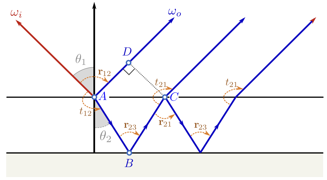
A thin film has two boundaries and three media (Fig. 3):

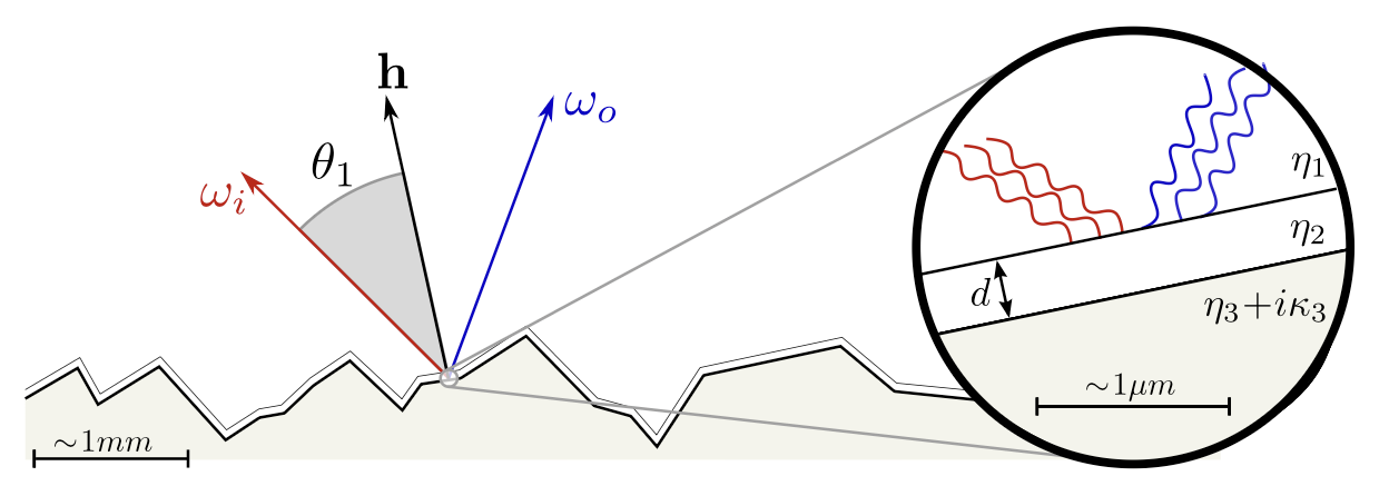
Multiple reflections inside the film interfere. The phase shift is

\Delta\phi = \frac{2\pi\mathcal{D}}{\lambda},\quad
\mathcal{D} = \eta_2(AB + BC) - \eta_1 AD,

and the (k)-th reflected amplitude:

r_k = t_{12} r_{23}\,(r_{21}r_{23})^{k-1} t_{21}\,e^{i k \Delta\phi}.

Summing all paths (Airy summation):

r = r_{12} + \sum_{k=1}^{\infty} t_{12} r_{23}(r_{21}r_{23})^{k-1}t_{21}e^{i k\Delta\phi}
= r_{12} + \frac{t_{12}r_{23}t_{21}e^{i\Delta\phi}}{1 - r_{21}r_{23}e^{i\Delta\phi}}.

For unpolarized light, the reflectance is

R = \frac{|r^{\perp}|^2 + |r^{\parallel}|^2}{2}. \tag{3}

Rendering

BRDF Model

Replace the Schlick Fresnel term in the Cook–Torrance microfacet BRDF with the Airy reflectance:

\rho(\omega_o,\omega_i) = \frac{D(\mathbf{h})\,G(\omega_o,\omega_i)\,F(\mathbf{h}\!\cdot\!\omega_i)}
{4(\omega_o\cdot\mathbf{n})(\omega_i\cdot\mathbf{n})},

wavelength-dependent:

\rho(\omega_o,\omega_i;\lambda)
= \frac{D(\mathbf{h})\,G(\omega_o,\omega_i)\,R(\mathbf{h}\!\cdot\!\omega_i;\lambda)}
{4(\omega_o\cdot\mathbf{n})(\omega_i\cdot\mathbf{n})}. \tag{4}

Spectral Integration

RGB renderers approximate spectral integration with three bands (R, G, B), mimicking the human eye’s LMS cones (Fig. 5):

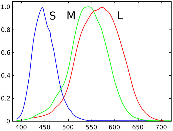
The per-band integrated reflectance:

L = \int_{0}^{\infty} S(\lambda)\,\overline{L}(\lambda)\,d\lambda,\\
M = \int_{0}^{\infty} S(\lambda)\,\overline{M}(\lambda)\,d\lambda,\\
S = \int_{0}^{\infty} S(\lambda)\,\overline{S}(\lambda)\,d\lambda.

L^{\uparrow}_j(\omega_o) = \int \frac{s_j(\lambda)}{\|s_j\|} L(\omega_o;\lambda)\,d\lambda,

L(\omega_o;\lambda) = \int_{\Omega} \rho(\omega_o,\omega_i;\lambda)\,L^{\downarrow}(\omega_i;\lambda)\,(\omega_i\cdot\mathbf{n})\,d\omega_i.

Pre-integrated:

L_j^{\downarrow}(\omega_i) = \int L^{\downarrow}(\omega_i;\lambda)\,\frac{s_j(\lambda)}{\|s_j\|}\,d\lambda,\\
\rho_j(\omega_o,\omega_i) = \int \rho(\omega_o,\omega_i;\lambda)\,\frac{s_j(\lambda)}{\|s_j\|}\,d\lambda.
``` \tag{5}

```math
L^{\uparrow}_j(\omega_o) \approx \int_{\Omega} \rho_j(\omega_o,\omega_i)\,L_j^{\downarrow}(\omega_i)\,(\omega_i\cdot\mathbf{n})\,d\omega_i.

And

R_j(\mathbf{h}\!\cdot\!\omega_i)
= \int R(\mathbf{h}\!\cdot\!\omega_i;\lambda)\,\frac{s_j(\lambda)}{\|s_j\|}\,d\lambda.

Analytical Spectral Integration of Reflectance

Starting from the Airy series:

r = r_{12} + \sum_{k=1}^{\infty} t_{12} r_{23}(r_{21}r_{23})^{k-1}t_{21}e^{i k\Delta\phi},

reparameterized:

r = \sum_{k=0}^{\infty} c_k e^{i\phi_k},

where

c_k = t_{12} r_{23}\,[r_{21}r_{23}]^{k-1} t_{21},\quad
\phi_k = k(\Delta\phi + \phi_{23} + \phi_{21}) - \phi_{21},

with (c_0 = -r_{21}) and (\phi_0 = \phi_{21}).

Then

|\mathbf{r}|^2 = \left|\sum_{k=0}^{\infty}c_k\cos\phi_k\right|^2
+ \left|\sum_{k=0}^{\infty}c_k\sin\phi_k\right|^2
= \sum_{k=0}^{\infty}c_k^2 + 2\sum_{k=0}^{\infty}\sum_{l<k}c_kc_l\cos(\phi_k-\phi_l),

defining (C_0 = \sum c_k^2), (C_m = \sum c_kc_{k+m}):

R = C_0 + 2\sum_{m=1}^{\infty}C_m\cos(m\Phi). \tag{6}

Closed-form:

R = R_{12} + R_{\star}
+ \frac{2\bigl(R_{\uparrow}\cos\Phi - R_{\uparrow}^2\bigr)}
{1 - 2R_{\uparrow}\cos\Phi + R_{\uparrow}^2}
\bigl(R_{\star} - \sqrt{T_{12}T_{21}}\bigr). \tag{7}

In frequency domain ((\nu=1/\lambda)):

R_j = \int \widehat{R}(\mu)\,\widehat{S}_j(\mu)^\star\,d\mu. \tag{8}

Finally

\boxed{
R_j = C_0 + 2\sum_{m=1}^{\infty}C_m
\begin{bmatrix}\cos(m\phi_2)\\\sin(m\phi_2)\end{bmatrix}^T
\begin{bmatrix}\Re_j(m\mathcal{D})\\\Im_j(m\mathcal{D})\end{bmatrix}
}. \tag{9}

Implementation

The implementation replaces the Fresnel term in the Cook–Torrance BRDF with the Airy spectral integration from Eq. (9). I based my code on the Mitsuba implementation, using a Gaussian approximation (or lookup table) for (\Re_j) and (\Im_j), with (m\in[1,3]). Transmittance (T) follows from (R+T=1).

I added a new material IridescentRoughConductor:

struct IridescentRoughConductor {
    Texture<Real> roughness;
    Texture<Real> anisotropic;
    Texture<Spectrum> film_texture;

    // Conductor
    Real eta;  // Real part of refractive index
    Real k;    // Complex part of refractive index

    // Thin film
    Real film_eta;       // IOR of thin film
    Real min_thickness;  // min height of thin film in nanometers
    Real max_thickness;  // max height of thin film in nanometers
};

Custom Scene

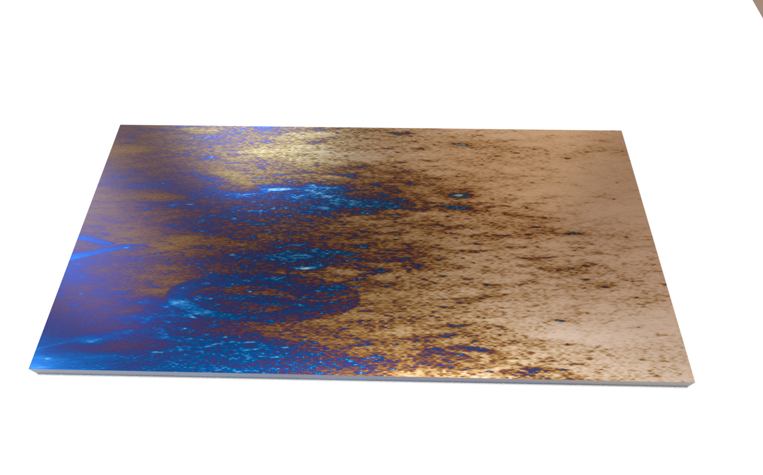
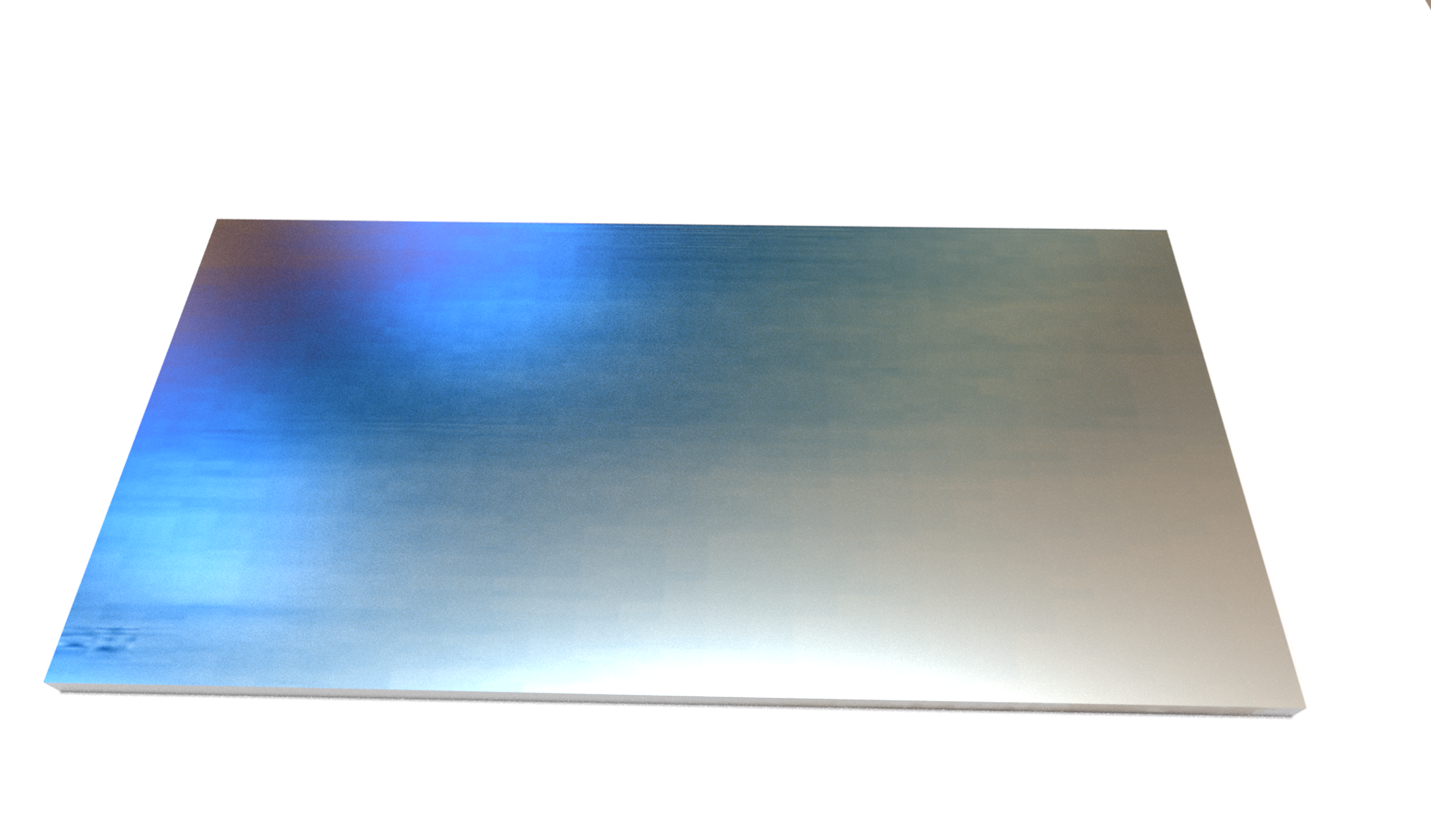
To demonstrate, I rendered differentially tempered steel (Wikipedia). Reference:

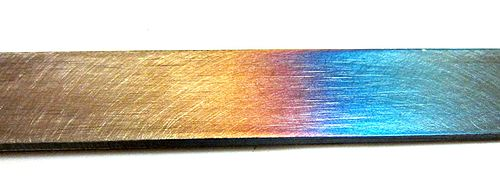
My renders:

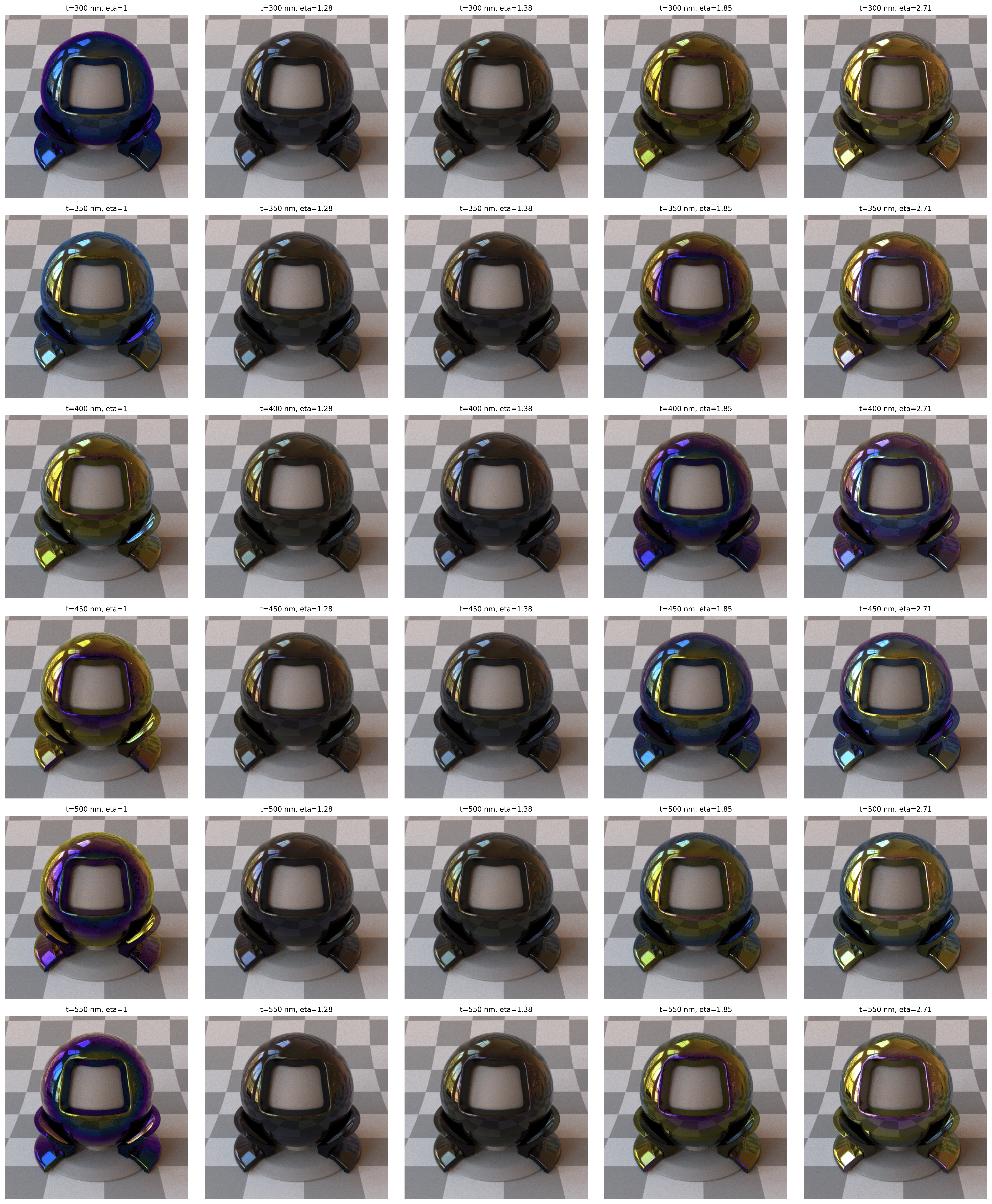
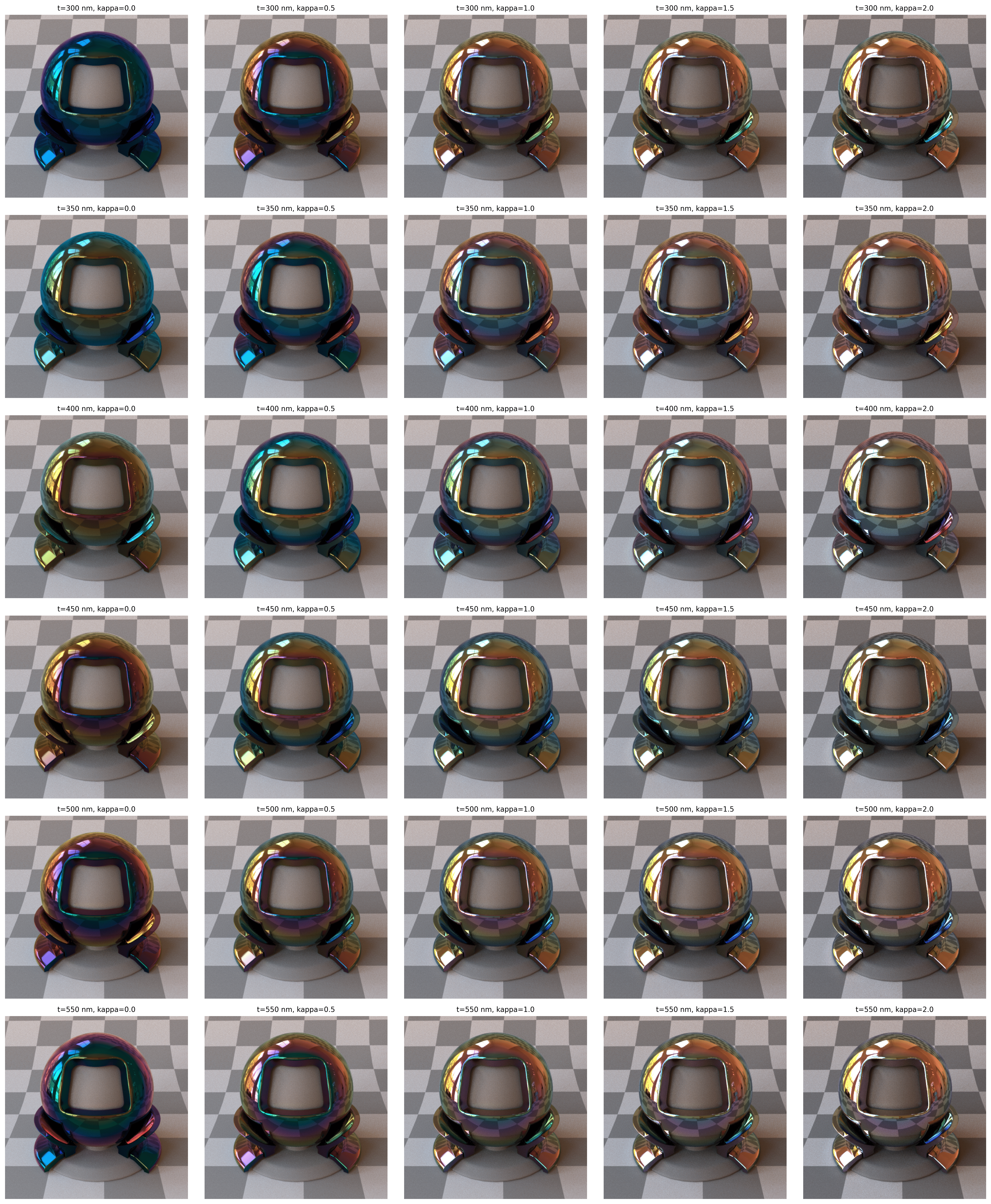
And parameter grids: